Natasha recently shared to me an interesting problem, sometimes asked in statistical interviews, which is surprisingly close to my own research field of graph theory. This particular problem appeared to be asked by Snapchat.
Consider boys and girls, each boy secretly loving a girl and vice versa. What is the probability that no couple could be formed?
An alternative mathematical formulation would be
Given two finite sets and , each containing elements, how many pairs of functions and are there, such that their composition has no fixed points?
The problem appears to be on OEIS and has two math.stackexchange entries with several very nice attempts. Apparently, my approach with generating functions seems to be new.
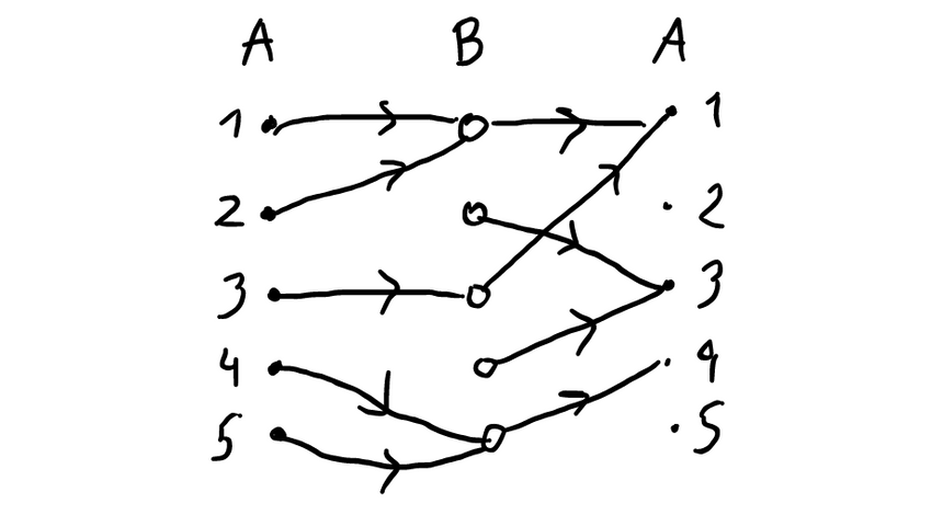
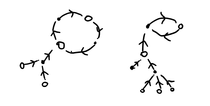
An example of a pair of functions with two mutual friendships 1-1 and 4-5. Each mutual friendship corresponds to a fixed point of the composition.
Previous works
Here is the link to the OEIS sequence of the first several terms
This OEIS entry also contains two links to Math StackExchange discussions

I personally love such kinds of problems because denoting the total number of endofunctions (i.e. functions from a set to itself) is also the number of rooted trees with one marked vertices. There are nice combinatorial bijections which can be used for asymptotic analysis.
Derangements
Let us start with an easier problem.
Given a finite set of size , how many functions are there without fixed points?
Clearly, for each of the points there are allowed possibilities of where the function would be pointing to. The number of functions is therefore . The probability that a randomly chosen function does not have fixed points is asymptotically
In this case, all the fixed points are formed independently, which is not the case in our problem.
Approach 1: exact formula and asymptotic analysis
Furthermore, if we look at the exact formula from OEIS, we observe
which I guess could be obtained by some kind of inclusion-exclusion. However, asymptotic analysis of such formulae may be sometimes difficult, while can still be useful for numerical simulations. In this case, however, asymptotic analysis is possible because the summands do not give increasingly divergent contributions.
Let us take a closer look at each of the summands as .
Note that is asymptotically , i.e. a polynomial of degree . The ratio is again a polynomial of degree , so when divided by the remaining part asymptotically does not depend on . The first several terms of this sum are approximately
With some extra work to make this proof rigorous we arrive to the answer .
Approach 2: conditional probabilities
Suppose that the items from the set receive, accordingly, incoming edges.
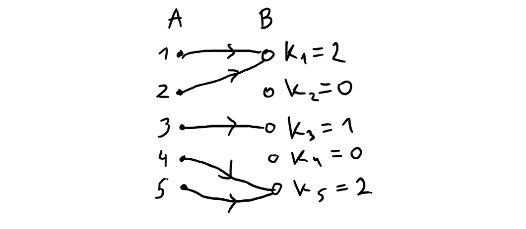
In this example, particular values of are given.
We can notice that since , we have for each . We could also compute and make sure it is finite (asymptotically does not depend on ). In fact each is distributed according to a Binomial distribution (although not independently) . Its variance is , and therefore, as .
First of all, suppose that all are equal to 1. Then, the probability that there are no mutual friendships is the same as in the derangements problem
Now, in the case of general , we replace the 1’s in the product by ’s:
By developing the Taylor series of the log, we obtain
This requires a better justification but heuristics says that on average, the answer does not depend on unless some of the is too large, which does not happen too often. By decomposing the probability up to conditional probabilities, we obtain
Approach 3: generating functions
Let us solve the derangement problem in a hard way first. From each node there is an arrow to another node. We look at the ensemble of arrows and nodes as a whole and try to find some structure in it.

It turns out that some nodes assemble into cycles, and others attach to nodes assembled as cycles. Everything outside the cycles forms trees ascending to one of the nodes of a cycle.
With some help of the exponential generating functions, we can express the combinatorial property that the endofunctions are sets of these cycle-trees (unicycles).
where is yet-to-be-determined exponential GF of unicycles. Since the exponential GF of cycles is just simply
the GF of unicycles could be obtained by a functional composition with the cycle function
where the generating function of rooted trees is defined by a recursive relation “a rooted tree is composed of a root and a set of rooted trees”:
This gives a surprising identity
I admit that being comfortable with this approach requires some experience. This is the reason I am trying to provide some more context and give more examples, which also takes more space. But the actual heuristic solution is very short, once all the intuitions are gained.
Remark. Joyal’s proof for the number of labelled trees .
The above approach allows to easily obtain the celebrated formula for the number of unrooted labelled trees . From the functional definition of the function , we get, by taking a pointed derivative
which is a linear equation that can be solved:
Therefore,
and it easily follows that the number of rooted trees is , so therefore, the number of non-rooted trees is divided by , which is .
Isolated cycles have Poisson distribution
The form of the generating functions allows one to obtain the Poisson distribution for the number of isolated cycles with almost no extra effort. Since the GF for all cycles is
we can mark the cycles of length 1 by introducing an extra variable :
The generating function of all the endofunctions with isolated cycles marked is now
The heuristics goes as follows:
Probability GF of the distribution is proportional to . To be fully rigorous, the probability GF is in fact , but the constant is distracting.
We would therefore expect that encodes a distribution, but it is not really clear what should be.
The asymptotic behaviour of generating functions is dictated by their singularities. In the general cases, these singularities play with each other, making the analysis more difficult, but in this particular case, we only need to know the value of at the singularity.
Since the singular expansion of gives , we therefore, conclude that and is the singularity closest to zero.
We often use the notation to denote th coefficient of the generating function .
But wait, we almost forgot about the factor in front and it is terrifying! But in order to get the probability generating function for the number of cycles, we can divide the counting GF by the total GF, just like in combinatorial probability, where we divide the number of “good” outcomes by the number of “total” outcomes.
and we know that the multiple will introduce some perturbation, but is a tiny guy (with asymptotically discrete distribution), so the final answer will not be changed. We, therefore, obtain, by some hand-waving
Remark. Further statistics by transfer theorems
The form of the generating functions also allows one to get the asymptotic distribution of previously unaccessible patterns. For example, we could ask for the distribution of the number of unicycles in the above graph. The answer comes by marking the unicycles with an extra variable:
Not so fast: the singular expansion of gives , and therefore, turns to infinity at , making the approach impossible. It would be still available if were a constant though!
We could still get the expected number of the cycles by using this approach.
The asymptotics of this generating function can be obtained by applying transfer theorems of Flajolet-Odlyzko. This is more or less a routine procedure and requires only the knowledge of these generating functions around their respective singularities.
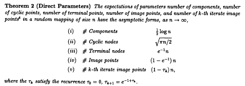
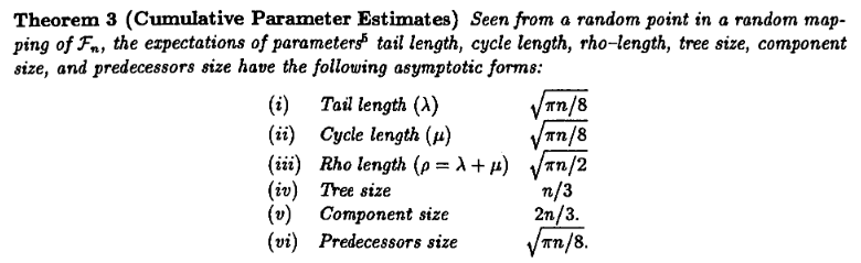
I invite the curious reader to check out a paper of Flajolet and Odlyzko entitled “Random mapping statistics” where they squeeze out everything that is possible to know about random mappings by a repeated application of the transfer theorem and the above symbolic method.
Composition of two mappings
Let us return to the original problem. It seems to be more difficult than just treating one mapping because now we have two mappings. But we will see that there is no need in applying transfer theorems at all, and a simple approach will do.
Now we have vertices of two colours, and we have to make sure that the arrows go between alternating colours.
We will use a variable for the vertices of the first colour, and for the vertices of the second.
The generating function of trees rooted at, respectively, the first or the second colour, would be
They, still, share the same singularity, but now it is trickier because in two dimensions, the singularity is not a single point, but a manifold. Well, if we require then the singularity would still be a point . In the end we need to make sure that the number of vertices of each colour is equal, which indirectly points to the symmetry and to the fact that in the heuristics.
Since in every cycle we have an even number of vertices, and black and white trees alternate, we therefore, have the generating function of cycles
Excluding the cycles of length 2 would mean cropping the first term in the expansion of the logarithm:
and the composition of two mappings now has a generating function with marking all the cycles of size , also corresponding to fixed points:
Note that the singular value of is again equal to 1 at the point .
As in the derangement exercise, we extract the coefficient and this gives us the probability generating function of the number of fixed points:
Final remarks
The trick above would not work if the number of black and white points is not equal. In this case, there is no guarantee that , and therefore, obtaining the singular point requires some more effort. No worries, saddle point analysis can help in this case.
Apparently, no paper analysing mapping statistics of the composition of two (or more?) mappings is published yet.
The same idea could be applied to the analysis of random graphs in stochastic block model. This is one of my research projects and I hope it can lead to some amazing discoveries. Even in the case of two parts (black points and white points?) there are vast unexplored terrains.